Chapter 11 kNN - k-nearest-neighbors

Very useful algorithm, identifies the k-nearest neighbors and classifies according to the majority vote of the neighbors.

kNN requires variables to be normalized or scaled. It is used to predict factor variables as well as continuous variables. In the caret implementation, the features, or the independent variables, can be both discrete and continuous.

# load libraries and look at the data
library(ISLR)
library(ggplot2)
library(caret)
library(Metrics)
head(Smarket)

##   Year   Lag1   Lag2   Lag3   Lag4   Lag5 Volume  Today Direction
## 1 2001  0.381 -0.192 -2.624 -1.055  5.010 1.1913  0.959        Up
## 2 2001  0.959  0.381 -0.192 -2.624 -1.055 1.2965  1.032        Up
## 3 2001  1.032  0.959  0.381 -0.192 -2.624 1.4112 -0.623      Down
## 4 2001 -0.623  1.032  0.959  0.381 -0.192 1.2760  0.614        Up
## 5 2001  0.614 -0.623  1.032  0.959  0.381 1.2057  0.213        Up
## 6 2001  0.213  0.614 -0.623  1.032  0.959 1.3491  1.392        Up

dim(Smarket)

## [1] 1250    9

s = Smarket
table(s$Direction)

## 
## Down   Up 
##  602  648

prop.table(table(s$Direction))

## 
##   Down     Up 
## 0.4816 0.5184

Now we fit the model

inTrain = createDataPartition(s$Direction, p = 0.75, list = FALSE)
training = s[inTrain,]
testing = s[-inTrain,]
fit = train(Direction ~ ., data = training, preProcess = c("center", "scale"), method = "knn")
fit2 = train(Direction ~ ., data = training, preProcess = c("center", "scale"), method = "knn", tuneLength = 6)

fit

## k-Nearest Neighbors 
## 
## 938 samples
##   8 predictor
##   2 classes: 'Down', 'Up' 
## 
## Pre-processing: centered (8), scaled (8) 
## Resampling: Bootstrapped (25 reps) 
## Summary of sample sizes: 938, 938, 938, 938, 938, 938, ... 
## Resampling results across tuning parameters:
## 
##   k  Accuracy   Kappa    
##   5  0.8385501  0.6754274
##   7  0.8457586  0.6896489
##   9  0.8475178  0.6931941
## 
## Accuracy was used to select the optimal model using the largest value.
## The final value used for the model was k = 9.

fit2

## k-Nearest Neighbors 
## 
## 938 samples
##   8 predictor
##   2 classes: 'Down', 'Up' 
## 
## Pre-processing: centered (8), scaled (8) 
## Resampling: Bootstrapped (25 reps) 
## Summary of sample sizes: 938, 938, 938, 938, 938, 938, ... 
## Resampling results across tuning parameters:
## 
##   k   Accuracy   Kappa    
##    5  0.8387262  0.6765276
##    7  0.8511159  0.7012801
##    9  0.8558962  0.7106913
##   11  0.8626060  0.7241337
##   13  0.8695310  0.7380914
##   15  0.8679743  0.7347562
## 
## Accuracy was used to select the optimal model using the largest value.
## The final value used for the model was k = 13.

plot(fit)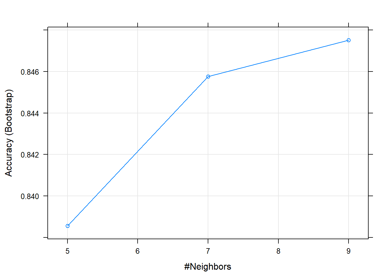

plot(fit2)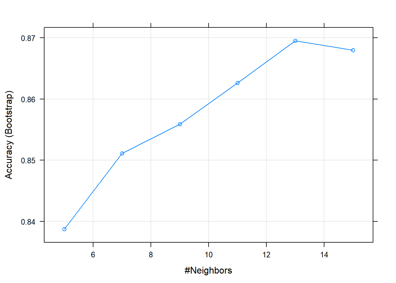

Let us check the accuracy of the model.

prediction = predict(fit, newdata = testing)
confusionMatrix(testing$Direction, prediction) #Actual data first, then the prediction vector

## Confusion Matrix and Statistics
## 
##           Reference
## Prediction Down  Up
##       Down  117  33
##       Up     11 151
##                                           
##                Accuracy : 0.859           
##                  95% CI : (0.8153, 0.8956)
##     No Information Rate : 0.5897          
##     P-Value [Acc > NIR] : < 2.2e-16       
##                                           
##                   Kappa : 0.716           
##  Mcnemar's Test P-Value : 0.001546        
##                                           
##             Sensitivity : 0.9141          
##             Specificity : 0.8207          
##          Pos Pred Value : 0.7800          
##          Neg Pred Value : 0.9321          
##              Prevalence : 0.4103          
##          Detection Rate : 0.3750          
##    Detection Prevalence : 0.4808          
##       Balanced Accuracy : 0.8674          
##                                           
##        'Positive' Class : Down            
## 

Let us try kNN for a continuous variable.

data(mtcars)
inTrain = createDataPartition(mtcars$mpg, p = 0.75, list = FALSE)
training = mtcars[inTrain,]
testing = mtcars[-inTrain,]
fit = train(mpg ~ ., data = training, preProcess = c("center", "scale"), method="knn")
fit

## k-Nearest Neighbors 
## 
## 25 samples
## 10 predictors
## 
## Pre-processing: centered (10), scaled (10) 
## Resampling: Bootstrapped (25 reps) 
## Summary of sample sizes: 25, 25, 25, 25, 25, 25, ... 
## Resampling results across tuning parameters:
## 
##   k  RMSE      Rsquared   MAE     
##   5  3.417859  0.7573906  2.785716
##   7  3.434295  0.7690902  2.803742
##   9  3.608257  0.7618139  2.927551
## 
## RMSE was used to select the optimal model using the smallest value.
## The final value used for the model was k = 5.

prediction = predict(fit, newdata = testing)
rmse(testing$mpg, prediction)

## [1] 4.133335

testing$predictedmpg = prediction
testing

##                     mpg cyl  disp  hp drat    wt  qsec vs am gear carb
## Datsun 710         22.8   4 108.0  93 3.85 2.320 18.61  1  1    4    1
## Valiant            18.1   6 225.0 105 2.76 3.460 20.22  1  0    3    1
## Merc 240D          24.4   4 146.7  62 3.69 3.190 20.00  1  0    4    2
## Merc 280           19.2   6 167.6 123 3.92 3.440 18.30  1  0    4    4
## Cadillac Fleetwood 10.4   8 472.0 205 2.93 5.250 17.98  0  0    3    4
## Toyota Corona      21.5   4 120.1  97 3.70 2.465 20.01  1  0    3    1
## Camaro Z28         13.3   8 350.0 245 3.73 3.840 15.41  0  0    3    4
##                    predictedmpg
## Datsun 710                29.08
## Valiant                   17.02
## Merc 240D                 23.16
## Merc 280                  20.88
## Cadillac Fleetwood        15.18
## Toyota Corona             27.56
## Camaro Z28                17.18